fortedata: Remote Sensing Data
Jeff Atkins
2021-05-16
Source:vignettes/fd_remote_sensing_vignette.Rmd
fd_remote_sensing_vignette.RmdRemote Sensing Background and Introduction
Multiple remote sensing technologies are being employed in FoRTE to collect data with the goal of creating a record of forest canopy structural and spectral change. These data are collected coincident with other data as outlined below (see Remote Sensing Methods). Canopy structure affects ecosystem functioning through altering light transmission/interception, subsequently affecting ecosystem functioning (e.g. productivity and the acquisition/use-efficiency of resources). See [the FoRTE Proposal Narrative] (https://fortexperiment.github.io/fortedata/articles/fd_forte_proposal_vignette.html) for further details.
Below we outline the remote sensing oriented data and functions included in fortedata.
Remote Sensing Functions
The fd_remote_sensing() script within fortedata currently includes the following functions:
fd_hemi_camera()returns a single data set that includes derived estimates of leaf area index, gap fraction, clumping index, and NDVI (normalized difference vegetation index) from terrestrial, upward-facing hemispherical photos looking into the forest canopy taken 1 meter above-ground (Table S9 in ESSD manuscript, Atkins et al. 2020).fd_canopy_structure()returns a single data set that includes 28 structural metrics estimating canopy structural traits such as height, area/density, openness, complexity, and arrangement. Data were processed usingforestrversion 1.0.1 (Atkins et al. 2018) in R Version 3.6.2.fd_ceptometer()returns a single data set that includes estimates of the fraction of photosynthetically available radiation (faPAR) absorbed by the canopy as well as leaf area index (LAI_cept)–each derived from a handheld ceptometer (LP-80; Decagon Devices) (Table S11 in Atkins et al. 2020).
Data Availability
fortedata is an evolving, open-science data package with data updated in near-real time. The current number of remote sensing data observations available as of 2021-05-16 are detailed in Figure 1.
no_of_records.df <- fd_observations()

no_of_records <- subset(no_of_records.df, table == 'fd_canopy_structure' | table == 'fd_hemi_camera')


ggplot2::ggplot(no_of_records, ggplot2::aes(x = as.factor(month), y = as.integer(year), fill= no_of_obs)) +
  ggplot2::geom_tile(ggplot2::aes(fill = no_of_obs), color = "black") +
  ggplot2::geom_text(ggplot2::aes(label = no_of_obs), color = "white") +
  ggplot2::coord_equal()+
  ggplot2::scale_fill_gradient(low = "#450d54", high = "#450d54", na.value = 'white')+
  ggplot2::scale_y_reverse()+
  ggplot2::theme_minimal()+
  ggplot2::theme(legend.position = "none")+
  ggplot2::ylab("Year")+
  ggplot2::xlab("Month")+
  ggplot2::ggtitle(paste("Figure 1: No. of observations currently available \nin each remote sensing function as of:", Sys.Date()))+
  ggplot2::facet_grid(table ~ .,  space = "free")+
  ggplot2::theme(strip.text.y = element_text(size = 9), strip.background = element_rect(
    color="black", fill="white", size= 0.5, linetype="solid"))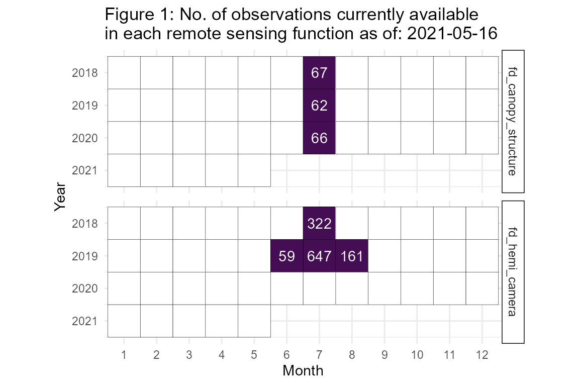
Remote Sensing Methods
Canopy Structural Traits (CSTs) from Terrestrial LiDAR
fd_canopy_structure() contains canopy structural trait metrics (Fahey et al. 2019) derived from 2-D terrestrial lidar data. These data were collected with a user-mounted, portable canopy LiDAR (PCL) system equipped with an upward facing, pulsed‐laser operating at 2000 Hz (Riegl LD90 3100 VHS; Riegl USA Inc., Orlando, Florida, USA). The PCL generates continuous LiDAR returns from a “slice” of the canopy as it is walked along a measured transect. For this study, we used 40 m transects at cardinal directions–north-to-south, east-to-west–through subplot center for a total of 80 m of transect length per subplot. This mirrors the approach of Atkins et al. (2018) and Hardiman et al. (2013) and is sufficient to account for spatial variability of forest structure (Hardiman et al. 2019). A more detailed description of the development and implementation of this terrestrial laser scanning system is available in Parker et al. (2004) and Hardiman et al. ( 2011). We derived canopy structural metrics using the forestr package (Atkins et al. 2018a, b) in R 3.5 (R Core Team, 2018). Data here are provided at the transect level, but should be averaged to make a plot mean.
data.frame(fd_canopy_structure_summary())
## These data are unpublished. Please contact Jeff Atkins to ask about using
## Data citation: ESSD
## Contact person: Jeff Atkins
## These data are unpublished. Please contact Jeff Atkins to ask about using
## Data citation: ESSD
## Contact person: Jeff Atkins
##    replicate year  rugosity rugosity_sd rugosity_n rugosity_se vai_mean
## 1          A 2018 29.608559   10.497869        129   0.9242858 6.796692
## 2          A 2019 29.735343    9.800674        139   0.8312823 5.996452
## 3          A 2020 24.637203   10.579291        135   0.9105204 6.953186
## 4          B 2018 22.436198    5.756363         70   0.6880170 7.232956
## 5          B 2019 23.611997    6.722365         81   0.7469295 6.520808
## 6          B 2020 22.069519    5.521884         86   0.5954400 7.053144
## 7          C 2018 14.014263    5.900967        109   0.5652101 6.695965
## 8          C 2019 14.580620    4.797647         93   0.4974929 5.941412
## 9          C 2020 14.931131    4.167939        105   0.4067492 5.929249
## 10         D 2018  9.080572    4.826094        121   0.4387359 5.832653
## 11         D 2019 10.567458    2.434255         78   0.2756251 5.259916
## 12         D 2020  8.748307    3.864607         91   0.4051209 4.780497
##    vai_mean_sd vai_mean_n vai_mean_se
## 1    0.8187640        129  0.07208815
## 2    0.9818119        139  0.08327619
## 3    0.6615754        135  0.05693934
## 4    0.3349234         70  0.04003100
## 5    0.5496304         81  0.06107005
## 6    0.5161193         86  0.05565458
## 7    0.5179845        109  0.04961391
## 8    0.5996817         93  0.06218410
## 9    0.5712212        105  0.05574548
## 10   1.0623365        121  0.09657604
## 11   0.8463590         78  0.09583129
## 12   1.4835040         91  0.15551347
## These data are unpublished. Please contact Jeff Atkins to ask about using
## Data citation: ESSD
## Contact person: Jeff Atkins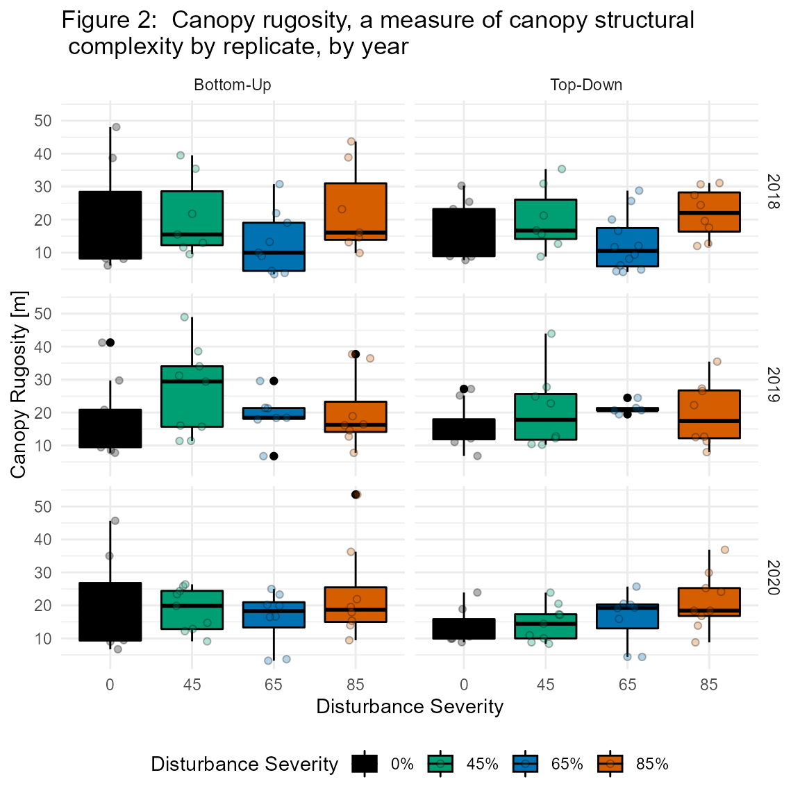
Hemispherical Camera Imagery
Below-canopy, hemispherical images were taken using a 24 Megapixel DSLR camera (Regent Instruments; Quebec, QU, Canda) with a 180° hemispherical lens during peak leaf-out (~July). The camera was facing-upwards, into the canopy and was mounted on a self-leveling tripod with the lens at 1 m from the ground. Leaf area index (LAICAM) was estimated using WinSCANOPY (Regent Instruments). Images were taken at all nested subplots (see fd_experimental_design_vignette).

Sample NDVI image

REU student Evan Paris taking images of the canopy using the NDVI camera
fd_hemi_camera()
## These data are unpublished. Please contact Jeff Atkins to ask about using
## Data citation: ESSD
## Contact person: Jeff Atkins## These data are unpublished. Please contact Jeff Atkins to ask about using
## Data citation: ESSD
## Contact person: Jeff Atkins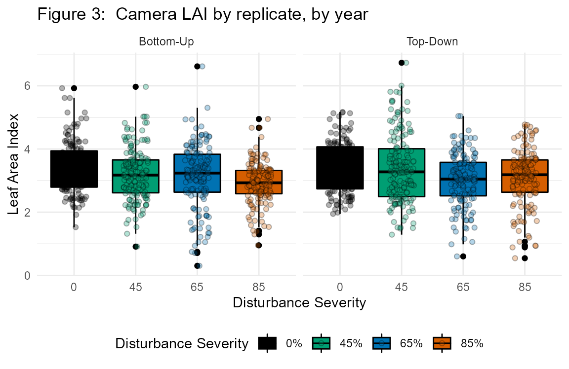
Light Interception
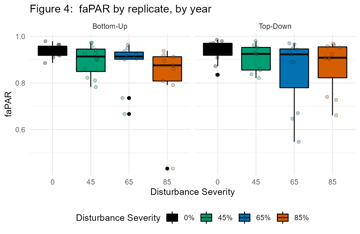
Light data–as fpar, the fraction of photosynthetically available radiation absorbed by the canopy–was acquired using a Decagon LP-80 handheld ceptometer (Decagon Devices; Pullman, Washington). fpar is the ratio of PAR above the canopy, to that measured below. fpar is assumed to be the difference between the two values. Below-canopy PAR measurements for each plot were taken along north-south and east-west transects (similar to PCL data above), with measurements taken every 1 to 3 m for a total of 30 - 60 measurements then averaged to make a subplot level mean of below-canopy PAR. Above-canopy PAR measurements were taken in open areas to ensure no interference from the canopy.
fd_ceptometer()
## # A tibble: 83 x 10
##    subplot_id replicate  plot subplot timestamp           a_par b_par fapar
##    <chr>      <chr>     <int> <chr>   <dttm>              <dbl> <dbl> <dbl>
##  1 D01W       D             1 W       2018-07-25 10:45:00 1276.  61.8 0.952
##  2 D03W       D             3 W       2018-07-25 10:56:00 1305.  98.3 0.925
##  3 D04W       D             4 W       2018-07-25 11:07:00 1305. 345.  0.735
##  4 D02W       D             2 W       2018-07-25 11:17:00 1367.  58   0.958
##  5 C04W       C             4 W       2018-07-25 11:24:00 1439.  40.6 0.972
##  6 C03W       C             3 W       2018-07-25 11:34:00 1383.  43.5 0.969
##  7 C02W       C             2 W       2018-07-25 11:45:00 1464.  49.5 0.966
##  8 C01W       C             1 W       2018-07-25 11:52:00 1475. 116   0.921
##  9 B04W       B             4 W       2018-07-25 13:25:00 1708.  61.7 0.964
## 10 B03E       B             3 E       2018-07-25 13:36:00 1768. 110.  0.938
## # ... with 73 more rows, and 2 more variables: lai_cept <dbl>, notes <chr>